Research perspective · 04
Virtual cohorts and the missing disease timeline
How tissue snapshots, sparse experiments, and clinical histories support different kinds of disease trajectories, and how to choose a useful starting point.
In an oncology dataset, baseline biopsies may be plentiful while repeat biopsies are scarce. Comparing responders with non-responders can identify different molecular states, but leaves a harder question open: how does a tumour move from one state to another?
Several computational approaches now address parts of that missing timeline. They can place samples along a progression sequence, estimate local changes in cell populations, or reconstruct the interval between experiments. Other models learn from years of clinical records and generate possible future histories or entirely synthetic cohorts.
These outputs are useful for different reasons. A progression model can suggest which patients to resample. A dynamic tissue model can identify an interaction worth perturbing. A synthetic cohort can make a longitudinal analysis easier to develop and share. Choosing among them starts with asking where the temporal information actually comes from.
1. Five tasks often grouped under “virtual cohorts”
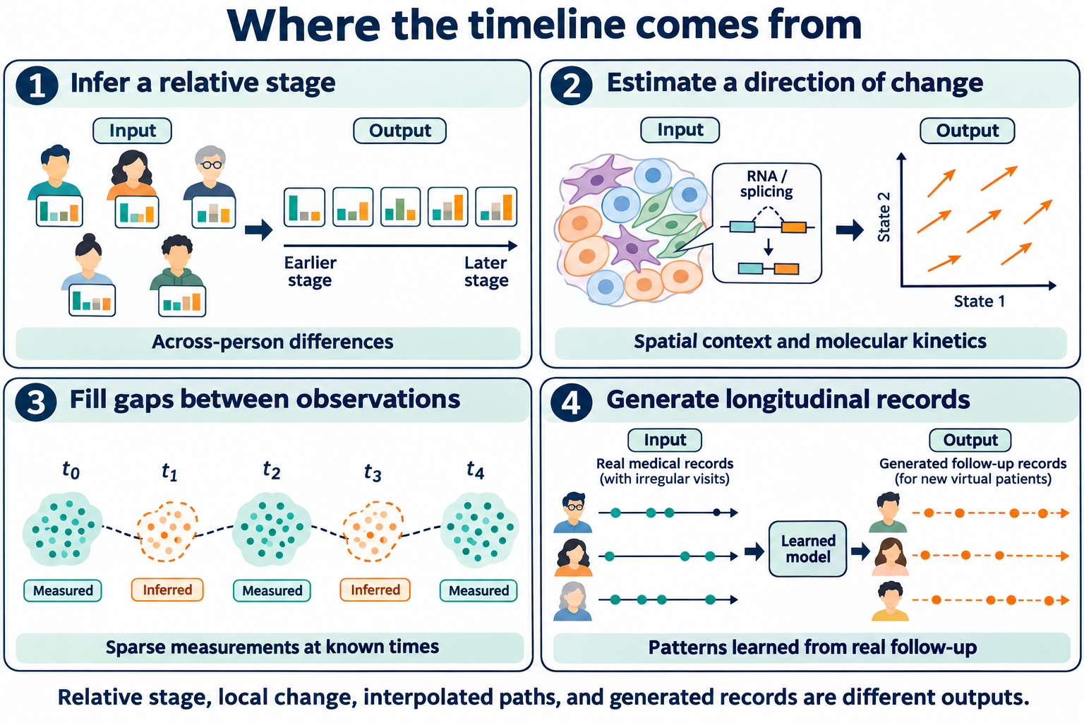
“Virtual cohort” is used broadly. Strictly, a synthetic cohort is a collection of generated patient records. A set of patients arranged by inferred disease stage is a different object: the people are real, while their placement on a common timeline is estimated. A simulated tissue trajectory has yet another unit of analysis.
| Task | Where time information comes from | Output | Examples |
|---|---|---|---|
| Infer progression stage | Differences in biomarker abnormalities across people | Relative order, stage, or progression subtype | Event-based models, SuStaIn, pseudo-longitudinal imaging [1]–[3] |
| Estimate local dynamics | Spatial neighborhoods, proliferation markers, or RNA-processing signals | A direction of change or a model of population dynamics | OSDR, VeloCD [4], [5] |
| Interpolate sparse measurements | Cell populations measured at several known times | Estimated paths between observed distributions | PROFET [6] |
| Forecast a patient's trajectory | Patterns learned from real clinical histories | Possible future events, measurements, or scores | Delphi-2M, DT-GPT [7], [8] |
| Generate a synthetic cohort | The distribution of real longitudinal records | New records intended to preserve useful population patterns | MeLD [9] |
The first three tasks can extract more information from incomplete observations. The last two depend on a training resource that already contains longitudinal structure. A person may need only one baseline measurement at prediction time even though the model learned its forecasting ability from many other people’s follow-up.
2. What can a snapshot tell us about change?
Spatial variation can help estimate local growth rules
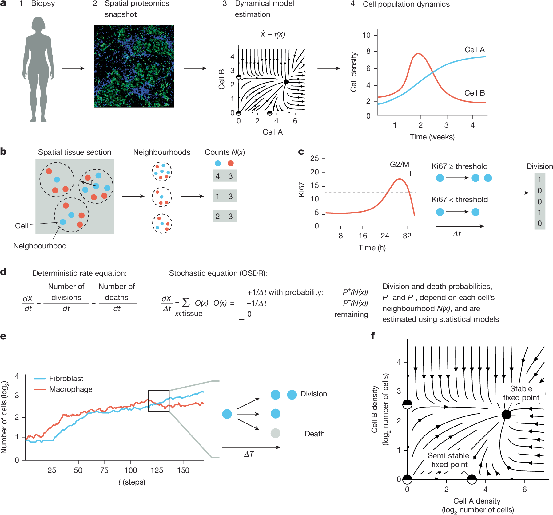
OSDR, described in Nature in 2026, uses cell identities, locations, and Ki67 division status to ask how neighborhood composition predicts proliferation. Spatially different neighborhoods supply examples of different local conditions. Estimated division and removal rules then drive tissue simulations.4
The removal term is important. Proliferation alone does not determine net population growth. The paper approximates each cell type’s removal rate by its mean division rate, an equality motivated by quasi-steady-state tissue. This assumption helps make snapshot-based dynamics estimable.
In NeoTRIP breast cancer data, models fitted separately to known responder and non-responder groups produced different tumour trajectories. That is evidence for studying response-associated tissue dynamics; independently predicting an unseen patient’s response requires a different evaluation.
For an omics study, the appealing idea is that variation within a specimen can help estimate a local response rule. It also suggests an experimental test: alter the neighborhood and measure whether the predicted change in growth occurs.
Across-person differences can reveal stage and subtype
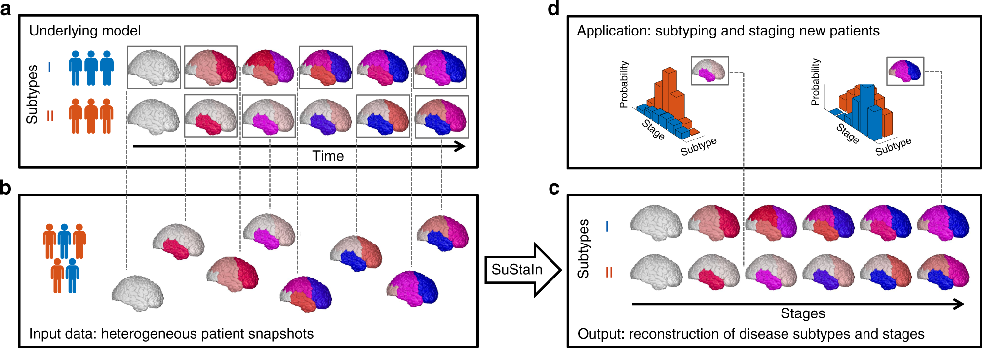
A complementary route asks which biomarker abnormalities tend to precede others across a population. Fonteijn and colleagues’ event-based model formalized this approach in 2012.1 SuStaIn later combined stage inference with subtype discovery, allowing different groups to follow different sequences of regional neurodegeneration.2
This addresses a common ambiguity in cross-sectional data. Two clusters may represent different disease pathways, or they may contain people observed at different stages of one pathway. Modeling subtype and stage together gives those explanations a way to compete.
Liang and colleagues provide a concrete pseudo-longitudinal example. They ordered 378 amyloid-positive participants by the extent of abnormal regional amyloid accumulation, then examined the inferred order against cognitive progression information.3 The resulting axis describes relative pathological burden. Converting a distance along that axis into elapsed years would require additional calibration.
In cancer, this distinction is particularly useful when interpreting a molecular trajectory: variation in treatment exposure, anatomical site, or tumour subtype can resemble progression. Those alternatives should be examined before assigning an early-to-late interpretation to a sample ordering.
RNA processing supplies a different kind of directional signal
VeloCD applies RNA-velocity reasoning to whole-blood transcriptomes. The relation between unspliced and spliced transcripts supplies information about expression change; reference disease-state data then support estimates of transitions toward clinical groups.5
The study tested day-one samples from controlled influenza and SARS-CoV-2 infection experiments with subsequent outcome measurements. The relevant analyses included 23 and 26 participants, respectively. Here, the temporal clue comes from molecular kinetics and the reference data, rather than from sorting people by a disease-burden score.
These approaches illustrate why “one sample” is an incomplete description of an experiment. A single sample can contain spatial structure or kinetic measurements that a conventional expression matrix does not retain. The assay and preprocessing must preserve the signal that the intended method uses.
3. Sparse time points can support a more detailed path
When several sampling times are available, the question changes. We already know that the population changed; we want to estimate how it moved between observations.
PROFET combines a particle-based reconstruction of expression trajectories with force matching to learn a smooth, time-dependent velocity field. In one benchmark, it learned from mouse embryonic stem-cell samples at 0, 24, and 48 hours, and was tested against the withheld 12- and 36-hour distributions. The paper also examined palbociclib response in breast cancer cells and patient datasets.6
That held-out-time design is worth borrowing. Matching the two endpoints leaves many possible paths between them. A withheld intermediate measurement asks whether the chosen path predicts something that was available to test but unavailable during fitting.
Destructive sequencing still samples different cells at each time. An inferred path connects population distributions under the model’s assumptions; identifying the actual ancestor of an individual cell needs additional lineage evidence. The reconstruction can nevertheless help locate a transition window for a follow-up experiment, such as the period when a resistant-like expression program begins to diverge.
This makes sparse longitudinal studies attractive on their own terms. A small number of carefully timed measurements can constrain a dynamic question more directly than a much larger collection taken at only one endpoint.
4. Clinical trajectory models learn from an existing time axis
Clinical records provide dates, repeated visits, treatments, and outcomes. Generative models can learn this structure, but their outputs serve different research purposes.
| Model | Learning strategy and output | Useful research role |
|---|---|---|
| Delphi-2M | A generative transformer predicts the next disease event and waiting time, then samples continued histories | Estimate disease risks and alternative event trajectories from prior history [7] |
| DT-GPT | A biomedical language model is fine-tuned on formatted clinical histories to forecast numerical trajectories | Predict future laboratory measurements or disease scores [8] |
| MeLD | A variational autoencoder represents mixed clinical variables; a diffusion model generates longitudinal records in latent space | Build synthetic cohorts for methods development and longitudinal analyses [9] |
Delphi-2M trained on roughly 400,000 UK Biobank participants and underwent external evaluation in Danish registry data. It generates distributions of possible histories, with explicit event timing.7 A forecast is therefore better understood as a set of possible continuations than as a fixed future chart.
DT-GPT examines a more numerical forecasting task. Its evaluations include laboratory trajectories over 13 weeks in non-small cell lung cancer, physiological measurements over 24 hours in intensive care, and cognitive scores over 24 months in Alzheimer’s disease. The targets and time scales differ across these evaluations.8
MeLD addresses a data-sharing problem. It learned from nearly 50,000 people living with HIV in CCASAnet, with records spanning more than 30 years. Its evaluation includes survival patterns, risk-factor associations, and privacy attacks, alongside general data resemblance. The synthetic data require an access application; the code is public.9
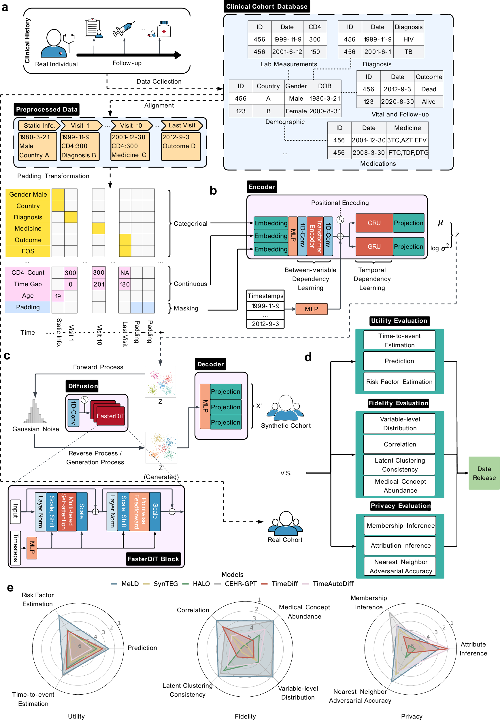
For a survival-analysis project, this last example changes what “realistic” should mean. Similar-looking laboratory distributions are insufficient if event timing, censoring, or their relation to patient characteristics is distorted. A useful synthetic dataset should preserve the relationships needed by the analysis being developed. Privacy also needs its own assessment; generated records are not automatically safe to release.
5. Choosing a useful project in oncology
The starting point should be the missing observation that would change the scientific conclusion. If the goal is to understand when resistance emerges, extra simulated patients will not by themselves answer it. If the obstacle is sharing a complicated longitudinal data structure, synthetic records may be exactly the useful output.
| Data in hand | A focused question | A useful next measurement or test |
|---|---|---|
| Baseline molecular profiles + outcomes | Does an inferred stage distinguish progression from molecular subtype? | Independent follow-up samples, with treatment and sampling-site information |
| Spatial tissue profiles + division markers | Which neighborhoods predict altered cell growth? | Perturb a proposed interaction or measure the population again |
| A few treatment-time scRNA-seq samples | When do response trajectories separate? | Withhold one measured time; then sample the predicted transition window |
| Repeated clinical visits + outcomes | Can a forecast transfer to another centre, or can synthetic records preserve a chosen analysis? | Evaluate on real held-out patients and reproduce the intended endpoint analysis |
One useful design would combine broad baseline coverage with a smaller, deliberately selected follow-up set. Baseline data identify candidate stages or divergent response patterns. Follow-up samples test the proposed ordering and help choose the next sampling window. The value of the model is then measurable: does it help place the limited observations where competing explanations differ?
The same principle connects virtual cohorts with biomedical world models. A timeline provides a way to describe change. Comparing interventions adds another requirement: evidence that the predicted changes respond correctly to an action. Routine treatment histories contain both treatment effects and the reasons clinicians selected those treatments, so forecasting success alone does not resolve that question.
My expectation is that useful virtual-cohort studies will often pair broad coverage with a small amount of targeted longitudinal evidence. Inferred stages can guide resampling, reconstructed paths can guide an experiment, and synthetic records can make a tested analysis reusable. Each output earns its value through the observation or research task it helps improve.
References and resources
- Fonteijn HM et al. An event-based model for disease progression and its application in familial Alzheimer’s disease and Huntington’s disease. NeuroImage 60, 1880–1889 (2012).
- Young AL et al. Uncovering the heterogeneity and temporal complexity of neurodegenerative diseases with Subtype and Stage Inference. Nature Communications 9, 4273 (2018).
- Liang L et al. Spatial-temporal interactions between white matter hyperintensities and multiple pathologies across the Alzheimer’s disease continuum. Alzheimer’s & Dementia 21, e70098 (2025).
- Somer J, Mannor S, Alon U. Temporal tissue dynamics from a spatial snapshot. Nature 650, 490–499 (2026). OSDR code.
- Dunican C et al. Predicting trajectories of illness using RNA velocity of whole blood. Nature Communications 17, 3652 (2026).
- Cheng YC et al. PROFET predicts continuous gene expression dynamics from scRNA-seq data to elucidate heterogeneity of cancer treatment responses. Cell Systems, 101710 (2026). Code.
- Shmatko A et al. Learning the natural history of human disease with generative transformers. Nature 647, 248–256 (2025). Delphi code.
- Makarov N et al. Large language models forecast patient health trajectories enabling digital twins. npj Digital Medicine 8, 588 (2025).
- Liang ZJ et al. Generating synthetic multi-national longitudinal cohorts for clinically grounded HIV research. Nature Communications 17, 7857 (2026).