Research perspective · 02
From pathology slides to survival predictions
A practical map of the pathology AI stack: what each tool does, how to choose foundation models, and how the pieces become a patient-level study.
A bulk RNA profile can tell us that immune-related genes are highly expressed. A pathology slide lets us ask where those immune cells sit: inside tumour nests, around their edges, or elsewhere in the tissue. That spatial context makes histology interesting for an omics study.
The practical challenge is turning a very large image into measurements we can connect to molecular profiles and patient outcomes. Open-source pathology tools cover most of that journey, but they work at different levels. A slide reader, a nuclear segmentation model, and a foundation model are not interchangeable. Knowing how they fit together makes the field much easier to navigate.
1. What pathomics measures
Pathomics turns tissue morphology into quantitative features. These can be explicit measurements, such as nuclear size, cell density, or distances between cell populations. They can also be learned representations extracted from image patches by a pretrained encoder.
The two routes answer different questions. To study immune exclusion, cell locations and tissue boundaries are useful measurements. To build a broad slide-level predictor, pretrained image features provide a practical starting point without requiring exhaustive cell annotations. A strong image embedding does not automatically give us a cell count; a cell count does not capture everything in an image embedding.
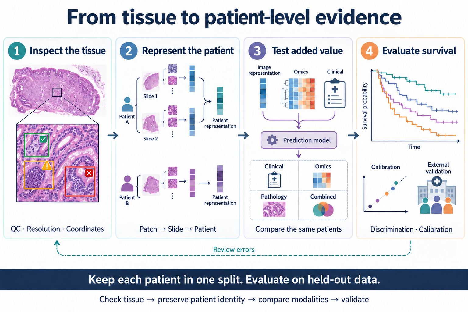
Both routes ultimately need a defined unit of analysis. Patches describe regions, slides describe specimens, and survival outcomes belong to patients.
2. The technical stack: five layers
The stack is easiest to understand by following what each step produces. Some packages span several layers, so this is a map of responsibilities rather than a rigid classification.
| Layer | What it does | Representative tools | What moves downstream |
|---|---|---|---|
| 1. Read and inspect | Read selected regions of large slides; review tissue and draw regions of interest | OpenSlide, QuPath | Accessible images, annotations, specimen identifiers |
| 2. Quality control and preparation | Inspect artifacts, identify tissue, and select patch locations | HistoQC, GrandQC, TIAToolbox, TRIDENT | Tissue masks, QC decisions, patch coordinates |
| 3. Measure and represent | Segment nuclei for explicit morphology, or encode patches for representation learning | HoVer-Net, CellViT, UNI, CONCH | Cell objects and spatial measurements, or patch embeddings |
| 4. Aggregate and model | Combine patches into slide or patient representations; optionally integrate omics | CLAM, MIL-Lab / Feather, TITAN, MCAT | Slide embeddings or task-specific predictions |
| 5. Evaluate and interpret | Compare models on patient-level tasks; inspect selected tissue regions and prediction errors | Patho-Bench, scikit-survival, QuPath | Performance estimates, interpretable findings, questions for follow-up |
3. Choosing tools within the stack
Start with slides that someone can inspect
OpenSlide provides programmatic access to whole-slide images; QuPath provides a workspace for viewing tissue, annotations, and image-analysis results.7 Together, they connect the computational pipeline to what a pathologist can actually review.
QC belongs before large-scale feature extraction. HistoQC supports slide quality assessment, while GrandQC provides models for tissue detection and artifact segmentation.1, 8 Keep the QC outputs alongside the features so that a failed prediction can be traced back to the specimen.
Use cell segmentation when the question needs cells
HoVer-Net and CellViT produce nuclear segmentations and classifications. These outputs support questions about nuclear morphology and the spatial distribution of cell populations.9 If the hypothesis concerns tumour–immune proximity, this route provides measurements that can be checked directly on the tissue. The original CellViT repository now directs new users to CellViT++.
For outcome prediction without a specific cell-level hypothesis, patch embeddings provide another route. Cell segmentation need not be a compulsory step in every slide-prediction pipeline.
Choose a processing framework before writing another one
TIAToolbox provides a broad API for image loading, preprocessing, inference, and visualization.10 TRIDENT is particularly useful when the immediate task is to process a slide collection into tissue masks, patch coordinates, and encoder features.1
These frameworks save different kinds of work. A flexible image-analysis project may benefit from TIAToolbox’s APIs. A cohort study comparing pretrained encoders can use TRIDENT to keep extraction organized across models. Keeping patch coordinates also makes it possible to return from a feature vector to its tissue location.
Separate representation extraction from outcome modeling
Multiple instance learning (MIL) combines many patches under a slide- or patient-level label. CLAM provides weakly supervised modeling and attention heatmaps; MIL-Lab brings several aggregation methods into one implementation and includes pretrained Feather models.3, 11
Feather is itself an attention-based MIL model. Reusing a pretrained aggregator can reduce how much must be trained on a small outcome cohort. A slide foundation model such as TITAN provides another source of pretrained slide representations. Neither route removes the need to match the patch encoder to the aggregator.
4. Foundation-model selection guide
The first distinction is between a patch representation and a slide representation. The second is whether the task needs image features alone or an image–text interface. Those decisions narrow the options before any benchmark ranking does.
| Model family | Representation / design | Useful starting point for | Practical consideration |
|---|---|---|---|
| UNI / UNI2-h | Self-supervised ViT patch encoders | General-purpose pathology features for downstream pooling and prediction | Request weight access; preserve the model-specific preprocessing recipe |
| CONCH | Pathology image–text model | Text-guided retrieval and zero-shot experiments, alongside image-feature extraction | Text prompts are part of the experiment; CONCHv1.5 is also used as a patch encoder in other pipelines |
| TITAN | Multimodal slide-level model | Pretrained whole-slide representations, retrieval, and slide-level transfer | Uses CONCHv1.5 features and spatial coordinates; its repository requires model access |
| Prov-GigaPath | Paired tile and slide encoders | Comparing tile-level and whole-slide representations within one model family | Specify which encoder is being evaluated; tile features alone are not the slide representation |
| Virchow2 | Self-supervised patch encoder | An alternative pathology backbone in a matched encoder comparison | Specify feature construction, not just the model name; TRIDENT exposes full and CLS-only variants |
| Phikon / Phikon-v2 | Self-supervised patch encoders | Frozen-feature and MIL experiments; Phikon-v2 includes a Transformers loading example | Public pretraining cohorts include TCGA; inspect overlap with the proposed evaluation cohort |
| H-Optimus-0 / 1 | Pathology image encoders | Another backbone family for task-specific comparison | Check access, preprocessing, and license for the exact release; family members have different terms |
| CTransPath | CNN–Transformer patch encoder | Reproducing earlier MIL pipelines and retaining a historical baseline | The original implementation uses a modified timm package; follow its extraction recipe |
For a first survival experiment, one available patch encoder plus a fixed aggregation strategy is enough to establish a baseline. To test pretrained slide transfer, compare TITAN or Feather with a task-trained aggregator. For text-based queries, CONCH addresses a different need. Patho-Bench supports matched downstream evaluations, including regularized Cox models on pooled features.2
There is no reason to run every model in the table. Choose candidates that test a specific difference, then keep the cohort and evaluation protocol fixed. An available checkpoint also needs an appropriate license; download access and permission for a particular use are separate checks.
5. A practical route from WSI to survival analysis
Step 1: Build the patient–specimen map
Start with a table linking patient IDs, slides, specimen dates, and outcome records. Define the prediction time and keep every slide from one patient in the same split. Review a small selection in QuPath and run QC before processing the full collection.
Step 2: Extract a reproducible feature set
After installing TRIDENT and obtaining access to the chosen encoder, its documented UNI example combines segmentation, patching, and feature extraction:
python run_batch_of_slides.py --task all \
  --wsi_dir ./slides --job_dir ./trident_output \
  --patch_encoder uni_v1 --mag 20 --patch_size 256
The outputs include tissue contours, patch coordinates, and feature files. Retain these with the extraction settings. The example settings belong to this encoder recipe; another model may require different patch sizes or transforms. For large collections, test storage throughput on a small batch before committing the full cohort. TRIDENT also provides local slide caching and multi-GPU options.1
Step 3: Produce one analyzable record per patient
Choose whether to pool patch features, use a pretrained slide aggregator, or train MIL for the outcome. Several slides from a patient require an explicit combination rule. Patho-Bench documents patient-level pooling, including constraints for models that use spatial coordinates.2
Fit a clinical baseline and a pathology model first. Add omics only after those routes work separately. This makes a fusion result interpretable: compare clinical-only, pathology-only, omics-only, and combined models on the same patients, rather than quietly changing the cohort when measurements are missing.
Step 4: Evaluate predictions and return to the tissue
Keep feature selection and risk thresholds within training data. Report discrimination with a censoring-aware evaluation, and inspect calibration if the model outputs absolute survival probabilities. C-index, time-dependent AUC, and Brier scores answer different questions.6
Then inspect failed cases and attention maps with a pathologist. A region dominated by a fold raises a processing question; a region containing an unexpected tissue compartment raises a biological one. A heatmap helps decide what to examine next, but does not by itself identify a mechanism.
6. Where pathology and omics become more interesting together
MCAT and PathOmics provide distinct examples of pathology–genomics modeling for survival; they are separate projects, not two names for one method.4, 12 HEST supplies paired histology and spatial transcriptomics, opening a complementary question: which molecular patterns are recoverable from morphology?5
The HEST figure below makes that pairing concrete. Panel b connects tissue processing to aligned molecular and image records. Panels c–e then show three uses of the same resource: testing image encoders, relating morphology to expression, and aligning image and molecular representations. These are useful intermediate tasks before asking whether an image–omics combination improves patient-level survival prediction.
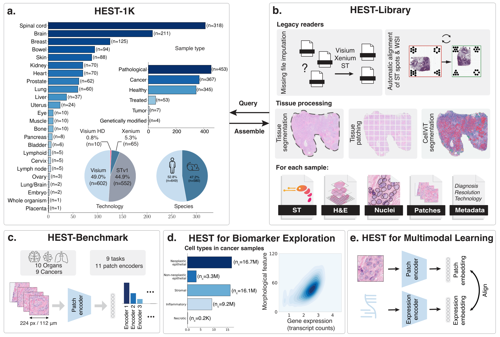
These routes can inform each other. A survival-associated image feature might correspond to tumour composition, stromal organization, or an immune-related spatial pattern. Paired molecular measurements can help distinguish those explanations and identify regions worth testing. That is a more informative follow-up than treating an improved fusion score as the endpoint of the study.
The tools make it feasible to move from slide inspection to patient-level prediction without building every component from scratch. A productive first study can use a modest stack: reliable QC, one encoder, a transparent aggregation choice, and a clinical comparison. More complex models become useful when they address something that baseline leaves unresolved, whether it is spatial structure, molecular complementarity, or transfer to another centre.
References and resources
- HistoQC and TRIDENT. Slide quality control and whole-slide processing documentation.
- Patho-Bench. Downstream benchmarking and patient-level pooling.
- MIL-Lab / Feather. MIL implementations and pretrained aggregation models.
- MCAT. Multimodal Co-Attention Transformer for Survival Prediction in Gigapixel Whole Slide Images. ICCV (2021).
- Jaume, G. et al. HEST-1k: A Dataset for Spatial Transcriptomics and Histology Image Analysis. NeurIPS (2024). Code and resources.
- Evaluating survival models. scikit-survival documentation.
- OpenSlide and QuPath. Whole-slide reading and interactive image analysis.
- GrandQC. Tissue detection and artifact segmentation.
- HoVer-Net and CellViT. Nuclear segmentation and classification.
- TIAToolbox. Image-processing, inference, and visualization APIs.
- CLAM. Weakly supervised modeling and attention visualization.
- PathOmics. Pathology-and-genomics Multimodal Transformer for Survival Outcome Prediction. MICCAI (2023).